Introduction to Control Barrier Functions
Introduction
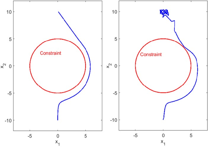
Obstacle avoidance is a fundamental and pervasive challenge in the design of control systems, with applications ranging from autonomous vehicles to robotic manipulators. At its core, the problem involves ensuring that a system navigates its environment without colliding with obstacles, which can often be represented as geometric constraints, such as ellipses or other shapes. These constraints are inherently rigid—for instance, a system must not enter a region defined by an obstacle. In optimal control problems (OCPs), such constraints are typically imposed as \(h > 0\), where \(h\) represents a safety condition. However, this formulation, while mathematically straightforward, often fails to account for the dynamic behavior of the system, leading to solutions that are neither safe nor robust. For example, minimizing control effort might result in trajectories that come dangerously close to obstacles, leaving little margin for error in the presence of uncertainties or disturbances.
To address this limitation, researchers have explored innovative approaches that incorporate additional system dynamics, such as velocity, into the constraint formulation. These methods aim to make the safety condition more sensitive to the system’s behavior, ensuring that the system not only avoids obstacles but does so in a manner that is dynamically feasible and robust. This line of inquiry has culminated in the development of Control Barrier Function (CBF) Theory, a powerful framework that transforms rigid safety constraints into dynamic, system-aware conditions. By leveraging CBFs, we can construct new constraint terms that are explicitly tied to the system’s dynamics, enabling safer and more efficient control strategies. This article delves into the principles of CBFs, their application in obstacle avoidance, and their role in advancing the field of control system design.
CLF
we consider an affine system:
\[\dot{x} = f(x) + g(x)u\]we have V as Lyaponov funtionc:
\[\begin{align} \dot{V}(x,u) &= \nabla V(x) \cdot \dot{x} \\ &= \nabla V(x) f(x) + \nabla V(x) g(x) u \\ &= L_f V(x) + L_g V(x)u \end{align}\]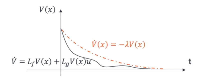 exponentially stabilizing CLF
so it would be :
\[\dot{V}(x,u) + \lambda V \leq 0 \quad \text{or} \; \delta \; \text{for relaxation}\] \[\begin{cases} V_1(x_c(t)) = (\upsilon_c(t) - \upsilon_d )^2\\ V_2(x_1(t)) = (\upsilon_1(t) - \upsilon_d )^2\\ V_3(x_c(t)) = (y_c(t) - l )^2\\ V_4(x_1(t)) = (y_1 - l )^2 \end{cases}\] \[\begin{equation} \begin{bmatrix} x_i \\ y_i \\ \theta_i \\ \dot{v}_i \end{bmatrix} = \begin{bmatrix} v_i \cos \theta_i \\ v_i \sin \theta_i \\ 0 \\ 0 \end{bmatrix} + \begin{bmatrix} 0 & -v_i \sin \theta_i \\ 0 & v_i \cos \theta_i \\ 0 & v_i / L_w \\ 1 & 0 \end{bmatrix} \begin{bmatrix} u_i \\ \phi_i \end{bmatrix} \end{equation}\] \[\begin{equation} \begin{cases} 2(v_C(t) - v_d)u_C(t) + m_1(v_C(t) - v_d)^2 \leq \delta_1(t), \\ 2(v_1(t) - v_d)u_1(t) + m_2(v_1(t) - v_d)^2 \leq \delta_2(t), \\ 2(y_C(t) - l)(v_C\sin\theta_C + v_C\cos\theta_C \cdot \phi_C) + m_3(y_C(t) - l)^2 \leq \delta_3(t), \\ 2(y_1(t) - l)(v_1\sin\theta_1 + v_1\cos\theta_1 \cdot \phi_1) + m_4(y_1(t) - l)^2 \leq \delta_4(t). \end{cases} \end{equation}\]llBF
for finding safe region we use the dual of CLF:
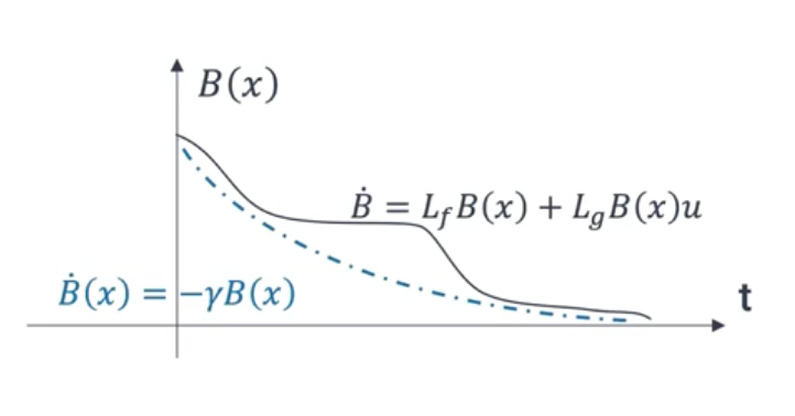 exponentially stabilizing CBF
CBF
go an use kappa functions
\[\begin{equation} \begin{cases} b_{C,H} = \dfrac{(x_C(t) - x_H(t))^2}{a_C^2} + \dfrac{(y_C(t) - y_H(t))^2}{b_C^2} - v_C^2(t) \geq 0, \\[10pt] b_{1,C} = \dfrac{(x_1(t) - x_C(t))^2}{a_1^2} + \dfrac{(y_1(t) - y_C(t))^2}{b_1^2} - v_1^2(t) \geq 0, \\[10pt] b_{1,H} = \dfrac{(x_1(t) - x_H(t))^2}{a_1^2} + \dfrac{(y_1(t) - y_H(t))^2}{b_1^2} - v_1^2(t) \geq 0, \\[10pt] b_{U,C} = \dfrac{(x_U(t) - x_C(t))^2}{a_C^2} + \dfrac{(y_U(t) - y_C(t))^2}{b_C^2} - v_C^2(t) \geq 0. \end{cases} \end{equation}\] \[\begin{align} L_f b_{C,H} (\mathbf{x}_C, \mathbf{x}_H) &= L_f b_{C,H} (\mathbf{x}_C, \bar{\mathbf{x}}_H + \mathbf{e}) \notag \\ &= \frac{2 (x_C - \bar{x}_H - e_x)}{a_C^2} (v_C \cos\theta_C - \bar{v}_H \cos\bar{\theta}_H - h_x - \dot{e}_x) \notag \\ &\quad + \frac{2 (y_C - \bar{y}_H - e_y)}{b_C^2} (v_C \sin\theta_C - \bar{v}_H \sin\bar{\theta}_H - h_y - \dot{e}_y), \end{align}\] \[\begin{align} L_g b_{C,H} (\mathbf{x}_C, \mathbf{x}_H) &= L_g b_{C,H} (\mathbf{x}_C, \bar{\mathbf{x}}_H + \mathbf{e}) \notag \\ &= [L_{g_u} b_{C,H} (\mathbf{x}_C, \mathbf{x}_H), L_{g_\phi} b_{C,H} (\mathbf{x}_C, \mathbf{x}_H)] \notag \\ &= 2 v_C \left[ -1, \frac{-(x_C - \bar{x}_H - e_x)}{a_C^2} \sin\theta_C + \frac{(y_C - \bar{y}_H - e_y)}{b_C^2} \cos\theta_C \right], \end{align}\] \[\begin{equation} \alpha_1 \big( b_{C,H} (\mathbf{x}_C, \mathbf{x}_H) \big) = k_1 b_{C,H} (\mathbf{x}_C, \bar{\mathbf{x}}_H + \mathbf{e}). \end{equation}\] \[\begin{equation} \begin{split} \frac{2 (x_C - \bar{x}_H - e_x)}{a_C^2} (v_C \cos\theta_C - \bar{v}_H \cos\bar{\theta}_H - h_x - \dot{e}_x) \\ + \frac{2 (y_C - \bar{y}_H - e_y)}{b_C^2} (v_C \sin\theta_C - \bar{v}_H \sin\bar{\theta}_H - h_y - \dot{e}_y) \\ + 2 v_C \left[ -1, \frac{-(x_C - \bar{x}_H - e_x)}{a_C^2} \sin\theta_C + \frac{(y_C - \bar{y}_H - e_y)}{b_C^2} \cos\theta_C \right] \\ + k_1 b_{C,H} (\mathbf{x}_C, \bar{\mathbf{x}}_H + \mathbf{e}) \geq 0 \end{split} \end{equation}\]Class \(\kappa\) functions are strictly increasing, continuous functions \(\kappa: [0, \infty) \to [0, \infty)\) with \(\kappa(0) = 0\). These functions are commonly used in control theory, Lyapunov stability analysis, and robust control.
Examples of Class \(\kappa\) Functions:
Linear Function: \(\kappa(r) = ar, \quad a > 0\) This is the simplest form, where (a) is a positive constant.
Power Function: \(\kappa(r) = ar^b, \quad a > 0, \quad b > 0\) This is frequently used in control applications.
Exponential Function: \(\kappa(r) = a(e^{br} - 1), \quad a > 0, \quad b > 0\) This function grows faster than polynomial functions.
Logarithmic Function (for small ( r )): \(\kappa(r) = a \ln(1 + br), \quad a > 0, \quad b > 0\) This is only a Class (\kappa) function for ( r \geq 0 ), as it is strictly increasing and satisfies (\kappa(0) = 0).
Square Root Function: \(\kappa(r) = a\sqrt{r}, \quad a > 0\) This grows slower than linear but still satisfies the required properties.
Sigmoid-Type Function: \(\kappa(r) = \frac{r}{1 + r}\) This is bounded, so it is not typically used when unbounded growth is needed, but it satisfies the basic properties of a Class \(\kappa\) function.
HOCBF
A simple CBF would enforce: \(\dot{b}(x) + k \cdot b(x) \geq 0,\)
- If Car 1 is braking hard and Car 2 is accelerating, the relative velocity could cause a collision before the simple CBF constraint is violated. An HOCBF would define a sequence of functions \(\psi_0, \psi_1, \psi_2\) as follows:
- \(\psi_0(x) = b(x)\) (position constraint),
- \(\psi_1(x) = \dot{\psi}_0(x) + \alpha_1(\psi_0(x))\) (velocity constraint),
- \(\psi_2(x) = \dot{\psi}_1(x) + \alpha_2(\psi_1(x))\) (acceleration constraint).
The HOCBF ensures that: \(\dot{\psi}_2(x) + \alpha_2(\psi_2(x)) \geq 0.\)
ACBF
- If the system is approaching the boundary of the safe set too quickly, increase the gain k in \(k \cdot b(x)\).
- If the system is far from the boundary, decrease k to allow more flexibility.